HOW TO CUT A HOLE?
A COMPARATIVE ANALYSIS OF SOME VERY BASIC TOPOLOGICAL PROCEDURES USED IN ARTISTIC 3D MODELING
INTRODUCTION
Here I’m describing what a 3D modeler actually does when performing certain 3D modeling routines. I don't mean a description of what goes on in the mind of a 3D modeler (the cognitive process), or of what actually goes on in the software the 3D modeler uses (the implementation), but just a visual description of the actual steps a 3D modeler takes from X to Y, where X and Y are some topologies of the 3D model the 3D modeler is modeling.
In the following, the “procedures” are simply the descriptions of 3D modeling routines involving topologies of 3D models and performed by 3D modelers in their everyday 3D modeling tasks.
These procedures are presented here in an elaborated version of “Martin’s diagrams” (or “modeling diagrams” or “m-diagrams” or, simply, “diagrams”). I’m naming them after Johnson Martin (Martin, 2015), because it’s the best use of a similar visualization for this specific purpose that I know of.
The procedures presented here all operate on very simple and flat 3D models that are represented as simple 2D structures, but the m-diagrams can also be used for more complicated 3D models.
We’ll go step-by-step through several actual 3D modeling procedures (of cutting a hole on a plane), used by actual 3D modelers, and described (or, rather, performed) in their YouTube or other such tutorials. For references, see the chapter “References” below.
I’ll compare and analyze each of these procedures and offer, at the end, some draft conclusions about them.
These modeling procedures do not describe the creative aspects of 3D modelers’ work, nor do they explain (or guarantee) the artistic value of the result. But, analyzed properly, they can help 3D modelers make their routine work more efficient, by giving them insight into the logic of the operations used to solve certain common 3D modelling tasks.
They're also useful in learning 3D modelling (that is, in education): knowing well the standard basic routines (and their varieties) may help 3D modelers achieve easier those other, non-routine (i.e. creative) goals.
Nota bene also that the search for the “best” procedure for a given topological task does not (in any way!) prescribe to 3D modelers a certain “right” way of modelling. In other words, the results of the following analysis of the 3D modeling procedures are not normative, and in the chapter “Conclusions” below I’ll explain why.
Here I mostly ignore what terms like “vertices”, “edges”, “faces”, “polygons”, “topology”, etc. exactly mean in mathematical topology, graph theory, and computer science, even though I'm borrowing some of these concepts below. I also ignore how these concepts are implemented in a particular 3D modelling software.
I use these terms instead simply as names of visual elements with which a 3D modeler works in a 3D software during the modeling process (the phenomenology).
I base the presented models and the operations on Blender (the 3D software that I'm best familiar with), but the similar results could be derived from other software too, even though work with 3D models is often in subtle (but important) ways different from one software to another.
I do assume that the reader of this text has some practical experience in 3D modelling, particularly (but not necessarily) in Blender.
Finally, please let me know if you know of other and better versions of the presented procedures! In the chapter “Challenges” below I’ll specify two challenges: if you can solve one (or both), I’ll add your solution to this article and you as its author.
THE BASICS
A brief reminder of what “vertex”, “edge”, “face” (or “polygon”), “model”, “geometry”, “mesh”, and “topology” mean for 3D modelers working in a 3D software. I actually assume you already know this, so I'm not explaining it in detail here, offering you instead only a brief refresher.
“Vertices”, “edges”, and “faces” (or “polygons”) are the basic intuitive working units for users of 3D modeling softwares. The virtual 3D objects that 3D modelers operate with while modeling are made up of simple (or more complex) structures of these elements, presented to the 3D modelers visually and interactively, somewhat irrespective of the way they're actually implemented in the given 3D software (IMAGE 1).

IMAGE 1
Vertices, edges, and faces are combined into “geometries” (displayed as “meshes”), and these “geometries” build up the “models”.
A “geometry” of a 3D model is the actual specification of the structure of the model, where each of its vertices, edges, and faces acquires a certain value assigned to it (a certain vector or another numerical or logical value). The “geometry” also means all the relational and derived properties of this value assignment: once you set the values for each vertex, edge, and face, then the relations between them (the relative lengths of its edges, the angles, etc.) and the derived properties (areas of the faces, etc.) are also set.
A “mesh” of a 3D model is simply the visual representation of its geometry in a 3D software: the dots, lines, and the (shaded) planes that 3D modelers see and interact with in the viewports of their 3D applications while modeling.
A “model” (or, more precisely, a “3D model”) is any structure built up of one or more geometries.
Finally, a “topology” of a 3D model is the structural logic of its geometry, not confined to the actual metrics of that geometry, but something more general.
The interesting thing with the geometry and its topology is that you can change the geometry of a 3D model (its values and relations), but keep the topology (the logic of that structure).
For the relations between the geometry and the topology of a 3D model, consider the following four cases:
The 3D models in the first pair are “congruent”, that is the right model is derived from the left model by translation, rotation, or mirroring of the whole model (IMAGE 2.1). Most of the values of the geometry are preserved (for example, the individual lengths of the sides) and so are its relational values (for example, the angles). Its topology is also preserved.
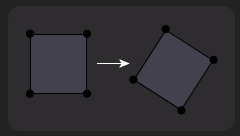
IMAGE 2.1
(2) The 3D models in the second pair are “similar”, that is the right model is derived from the left model by uniform scaling of the whole model (IMAGE 2.2). The relations of the geometry are again preserved (for example the angles), but the absolute values (the lengths) are changed. The topology is still preserved.
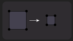
IMAGE 2.2
(3) The 3D models in the third pair are “homeomorphic” (more about this in the chapter “Procedures A, B1, B2, and B3”), that is, the right model is derived from the left model by deformations (moving the individual vertices around or non-uniform scaling or shearing) of the geometry such that the geometry is changed (even the relations change) but the topology is preserved (IMAGE 2.3).
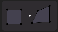
IMAGE 2.3
(4) The 3D models in the fourth pair are “non-homeomorphic”, that is, the right model is derived from the left model by changing the geometry in such a way (inserting new vertices and connecting them) that its topology is also changed (IMAGE 2.4).
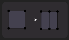
IMAGE 2.4
That's it for the basics!
M-DIAGRAMS
Now we'll develop the structure of the m-diagrams that we'll use to display and analyse several typical topological procedures of cutting a hole on a flat surface.
My inspiration for these diagrams comes from (Martin, 2015), but I've expanded them with some additional features that I found necessary for a more detailed analysis.
Suppose we wanted to model the topology Y starting from the topology X (IMAGE 3).
The question is "What modeling operations (and in what sequence) would we need to do in order to get from X to Y?" These two topologies (X and Y) are non-homeomorphic (see above), so the procedure we’re looking for profoundly alters the starting model to get us to the target model.
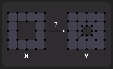
image 3
In Blender (but similarly in many other 3D modeling applications) we could proceed as follows:
(1) we select the inner edge loops of the model X,
(2) we extrude those inner loops, and
(3) we scale the edge loops of the extruded geometry inwards and we have the required model Y.
This can be written down as the following simple diagram, where X is the starting topology and Y is the result or target topology (IMAGE 4):
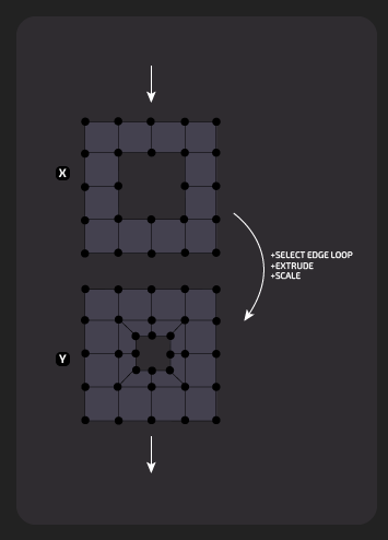
image 4
Now, important thing to notice here is that the operation on a topology is a function (of some sort) that takes some elements of the starting topology (vertices, edges, faces) as its arguments, and then does something with them (moves them, scales them, or modifies the topology in some other way). Therefore we'd like to have in the m-diagrams for such topological procedures a way of separating these “selection/operation steps” from the “result steps”.
If X and Y are the two topologies as above, then we could write the selection/operation as the step Z, something like this (IMAGE 5):
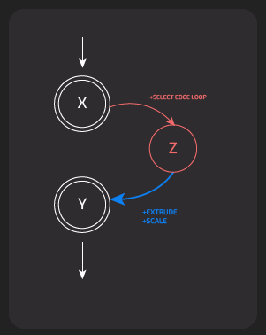
image 5
The diagrams for presenting topological procedures could thus be considered a kind of deterministic finite-state automata, describing a definite process from a start state (the starting topology) to the final state (the target topology). In graphs like these (IMAGE 6), we see that the topologies are the states of the automaton (with one start state and one final state) and the selections/operations are its step-by-step transitions:
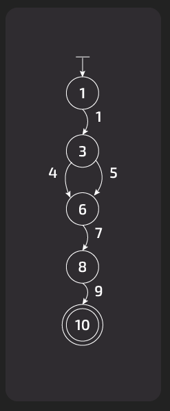
image 6
To be clear about what I mean by such a diagram, I present below (IMAGE 7) one complete topological procedure with the selection/operation plane separate from the result plane:
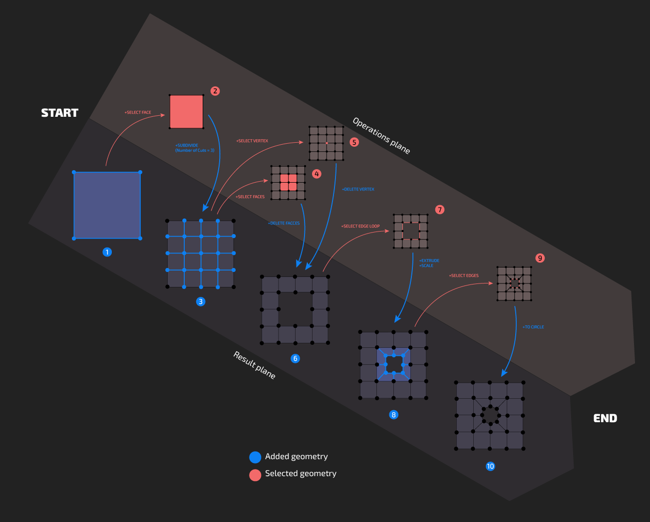
image 7
However, this is not graphically convenient, as it requires us to have two columns (two planes) for each procedure, and this doubles the graphical space needed.
Therefore, we could rewrite our procedure instead like this (IMAGE 8), with result and operation nodes alternating in a single column of the diagram:

image 8
The above diagram thus becomes the following diagram of a full topological procedure (IMAGE 9), and I call such a diagram an “m-diagram”:
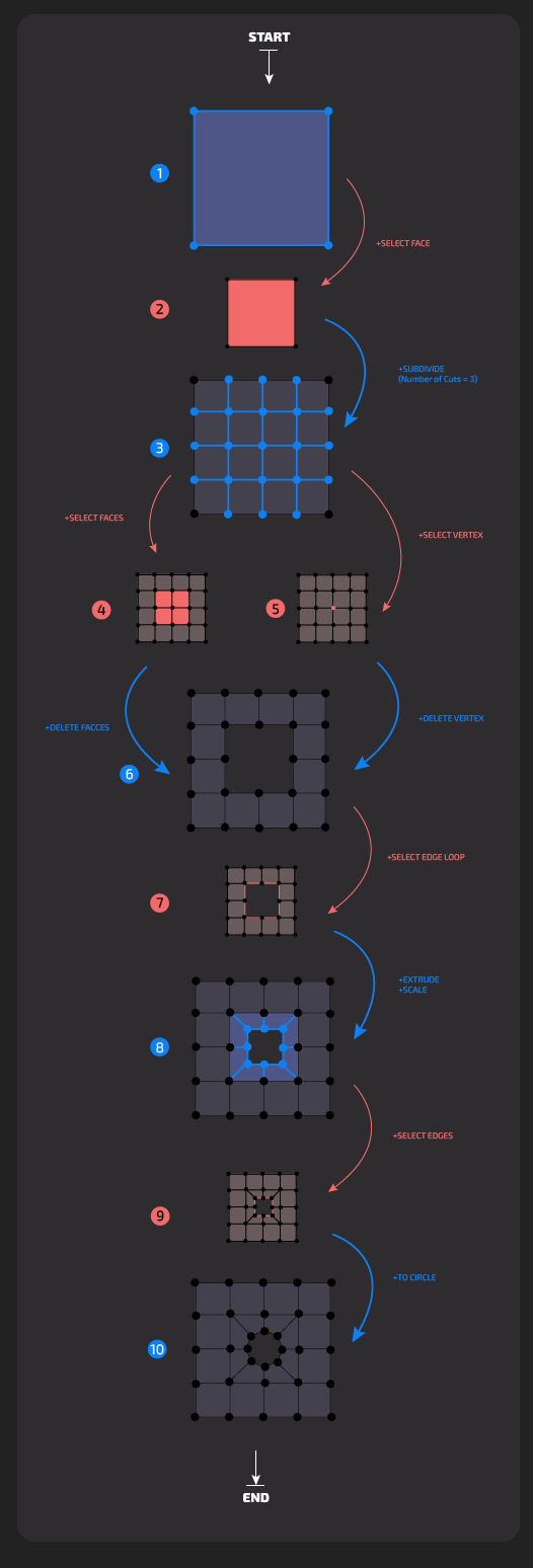
image 9
Now, the above m-diagram (IMAGE 9) of our procedure is not quite precise!
If we listed all the actual operations that take us to the resulting topology from the starting topology (i.e. the whole procedure), it would consists (in Blender) of more steps actually:
01. Add New Plane (Shift + A > Mesh > Plane)
02. Enter Edit Mode (Tab)
03. Choose Face Mode (3)
04. Select The Face (LMB Click)
05. Subdivide with 3 Cuts (RMB Click > Subdivide + Number of Cuts = 3)
06. Choose Vertex Mode (1)
07. Select A Vertex (LMB Click)
08. Delete The Vertex (X > Delete > Vertices)
09. Choose Edge Mode (2)
10. Select Edges (Alt + LMB Click)
11. Extrude (E)
12. Scale (S + Move)
13. Make Circular (Shift + Alt + S + Move)
But some of these steps we can easily ignore (for example the initial step of adding the starting topology).
Others (like entering Edit Mode, or switching between Vertex, Edge, and Face Edit Modes) are also implicit and so we can ignore them too.
Also, the details of shortcut keys pressed and mouse buttons clicked really depend on the way a 3D modeler set up his/her working environment (e.g. custom shortcuts, various wrapper add-ons, etc.), not to mention the differences between different 3D software the 3D modeler uses for these tasks.
Therefore, we can for now proceed with our m-diagrams as above, even though for more exact purposes a better and more precise account of the actual steps would be necessary.
PROCEDURES A, B1, B2, AND B3
So, in the following we'll be interested in the four procedures (A, B1, B2, and B3; IMAGE 9), that'll take us from the same starting topology of the model (a “quad” plane) to the target (or result) topologies of the model (a plane with a hole in it). This is a common simple task in 3D modeling: cutting a hole on a planar or curved topology.
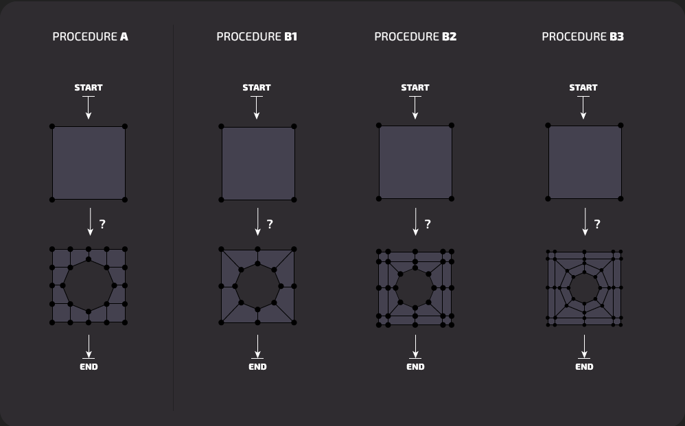
image 10
But why did I group the above four procedures (and the resulting topologies) in two major groups, A and B?
We can borrow from mathematical topology the notion of "homeomorphism" and use it here loosely (I know: one mathematician will die every time I use that term in what follows) to mean a class of topologies that can be transformed into one another by any modelling deformation, such as moving vertices, edges, or faces, or scaling or rotating them in any combination, but not by adding or removing or collapsing (fusing) or intersecting these elements.
For example, the first row below (IMAGE 11) presents few homeomorphic topologies, and the second row presents few non-homeomorphic topologies:
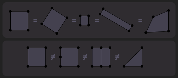
image 11
We can now see that there are two classes of topologies for our four procedures: Class-A and Class-B topologies, the members of each being mutually homemorphic. For example, in the first row below (IMAGE 12.1) two homeomorphic Class-A topologies are presented. In the second row three homeomorphic Class-B topologies are presented:
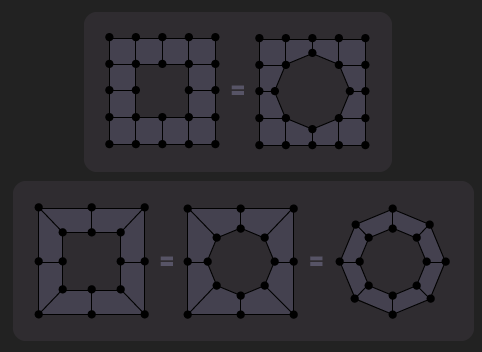
image 12.1
The topologies A (a Class-A topology) and B1 (a Class-B topology) are not homeomorphic, and neither are A and B2, or A and B3:
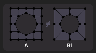
image 13
Furthermore, the topologies B1, B2, and B3 of the Class-B group of topologies are themselves not mutually homeomorphic:
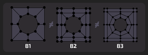
image 14
But topologies B2 and B3 have important subtopologies B2’, B3’, and B3’’ that are homeomorphic to the topology B1, so all three of the topologies (B1, B2, and B3) can be grouped as Class-B topologies because of this “embedding” (IMAGE 15.1):
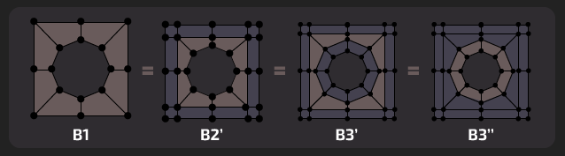
image 15.1
However, the outer subtopologies B2’’ and B3’’’ of the topologies B2 and B3 are homeomorphic to the topology A, so the topologies B2 and B3 have elements of both Class-A and Class-B topologies (IMAGE 15.2). But these outer subtopologies are only secondary or auxiliary: they only function as “isolators” of the central Class-B subtopologies (this is precisely what Arrimus 3D (Arrimus 3D, 2021) uses them for). Thus we can keep the topologies B2 and B3 in the Class-B group, together with B1.
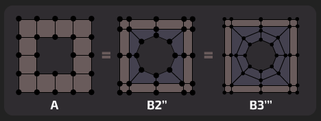
IMAGE 15.2
The other motivation for grouping the above topologies as Class-A and Class-B topologies is that, for some of the authors of the procedures below, Cédric Lepiller (Lepiller, 2020) and Arrimus 3D (Arrimus 3D, 2021), Class-A topologies perform better on curved surfaces than Class-B topologies, i.e. they behave differently when curved (and subdivided).
However, the most important takeaway here is that in creating the target topologies with our procedures A, B1, B2, and B3, in each case we’re radically transforming the starting topology of the model. That is, in all four procedures the starting and the result topologies are not homeomorphic.
Also, just to be clear, even though we're working here with flat (2D) topologies, all the above applies to the 3D configurations also, so that, for example, the Class-B topologies comprehend all of the following (and everything else derived by 3D deformations that keep these topologies homeomorphic):
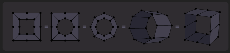
IMAGE 12.2
PROCEDURE A
Our first task then is to find a procedure A that'll take us from the starting topology (left) to the target topology (right):
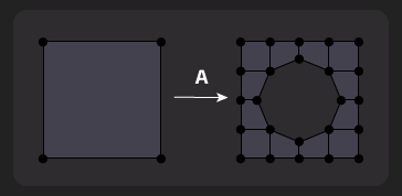
image 16
I’ll present here two versions of procedure A.
The first version (A.1) comes from Cédric Lepiller (Lepiller, 2020). Two things to mention here, before presenting the procedure.
First, in demonstrating his procedure, the author is using his own add-on for Blender, called “Speedflow”. But that addon is just an overlay (a wrapper) over standard Blender’s operations working under the hood, and so it’s easy to translate what it’s doing back to those underlying standard operations.
The other thing worth mentioning is that, in his video, Lepiller is specifically constructing a hole on a plane that will be bended (that is, a hole on a curved surface), so the resulting topology is intended to solve that specific problem. The other class of topologies (created by procedures B1, B2, and B3) would not, according to Lepiller, look as smooth when bended and subdivided. This is the mentioned other reason for my classification of the topologies into two main classes, Class-A and Class-B.
The second version (A.2) of the procedure A comes from the following presentations: Evermotion (Evermotion, 2013), Justin Geis (Geis, 2020), and Blender Secrets (Blender Secrets, 2020).
In contrast to Lepiller, these authors are not motivated (at least not directly) by the problem of creating a topology that’ll perform well when curved. However, even this problem aside, their version of the procedure A is shorter than Lepiller’s (a total of 9 modeling steps, compared to Lepiller's 19 steps), and would, to many 3D modelers, seem more intuitive and straightforward. Beside the need to curve the resulting topology, Lepiller might have presented a more complicated procedure because he wanted to demonstrate to his audience how his add-on works.
Anyway, here are the two versions of the procedure A, side by side (IMAGE 17):
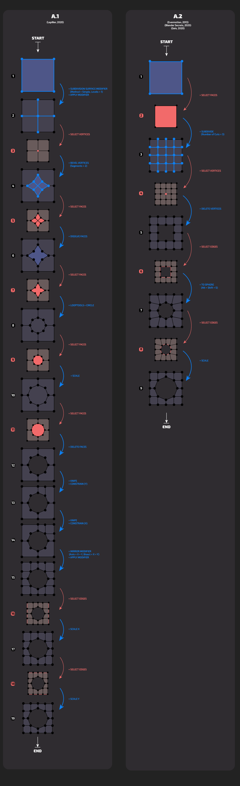
image 17
The first thing done in both of the versions (A.1 and A.2) is the subdividing of the initial topology.
While Lepiller in A.1 adds only one subdivision cut, the authors of A.2 are adding more cuts (=3) and thus seemingly create a more complex topology (consisting of more elements and their relations).
However, in the following it turns out that Lepiller in A.1 actually does a more complicated procedure of beveling the central vertex, and consequently has much more steps, with more complicated topological situations, than A.2.
Another thing to note here is that Lepiller in A.1 adds his initial cut by adding, setting the parameters, and then applying a Subdivision Surface modifier, operating on the whole model (i.e. no selection needed). The authors of A.2 select the face, and then use the plain Subdivide operation with certain parameters (number of cuts). While in this initial step Lepiller does without the additional selection step, he does so by using a modifier (with the whole deal of setting it up and then applying it) for the simplest possible task (adding one center vertex, connected to its projections on each side). Lepiller is perhaps overdoing what has to be done. But anyway, which is more complicated (Subdivision Surface modifier or the Subdivide operation) depends largely on either how each is implemented in a particular 3D software, or on the habits of a particular 3D artist modeling the model. More about this in the chapters "Discussion" and "Conclusions" below.
Also, A.1 is evidently longer than A.2. The easiest and most obvious (but somewhat misleading) way to compare two procedures (or two versions of the same procedure) is to count the total number of steps it takes each to reach the target topology from the starting topology, and then call the shorter one more effective. While in many cases this is true, it can be misleading, because length of a procedure alone does not account for certain specifics of the habits and preferences of the 3D modeler performing that procedure. Again, I’ll discuss this issue in detail below, in the chapters “Discussion” and “Conclusions”.
Note that the presentation A.1 of A is not entirely correct: in steps 8, 6, and 10 the selection is not lost in Blender when rounding or scaling, so the following step (where we re-select that area) is redundant (see the chapter “Discussion” below). However, procedure A.1 is still, even with these redundancies removed, longer and more complicated than procedure A.2.
Procedure A.2 is perhaps a canon for this particular task, as it’s more efficient and more authors use it. But this is controversial, or, at least, should not be normative.
PROCEDURE B1
Now we need to solve the following task. We need to find a procedure B1 that’ll take us from the starting topology (left) to the target topology (right):
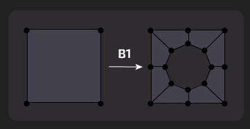
image 18
I’m presenting three versions (B1.1, B1.2, and B1.3) of the procedure B1.
The first one is again by Cédric Lepiller (Lepiller, 2020), the second by Blender Time (Blender Time, 2019A) and (Blender Time, 2019B), and the third is an alternative to B1.1 and B1.2 by Arrimus 3D (Arrimus 3D, 2021).
Lepiller’s version is only mentioned in his tutorial (Lepiller, 2020), but is very similar to his procedure A.1, so we can guess what it has to look like.
Here they are (IMAGE 19):
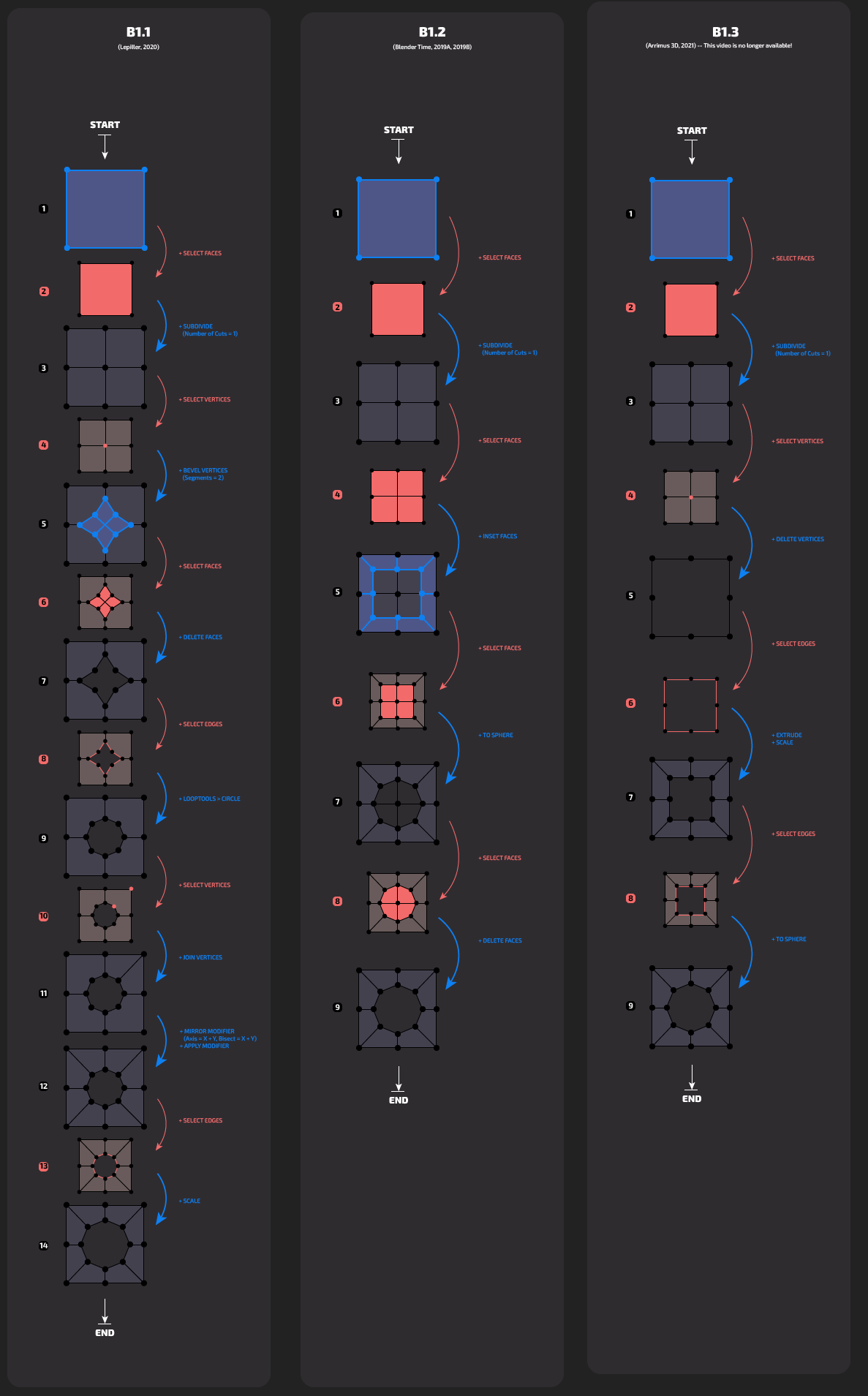
image 19
Lepiller’s procedure B1.1 has all the shortcomings of his procedure A.1 discussed above, so I won’t go into details about that here.
But if we mutually compare the procedures B1.2 and B1.3, then, even though these procedures have exactly the same number of steps, B1.3 is simpler because in its steps 4, 6, and 8 it requires you to select continuous the edge loop (one click with the Alt key pressed), and B1.2 is more complicated, because in the corresponding steps 4, 6 and 8 it requires you to select 4 faces one-by-one. Each of those three steps (4, 6 and 8) of B1.2 can be expanded to a sequence of four steps actually. More about this below, in the chapter “Discussion”.
PROCEDURE B2
Let's now solve the following task: we need to find a procedure B2 that’ll take us from the starting topology (left) to the target topology (right):
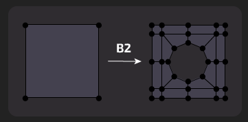
image 20
I present first the procedure B2.1, a solution by Arrimus 3D (Arrimus 3D, 2021).
Arrimus 3D is here creating a Class-B topology (similar to B1 and B3), but with support edge loops at the outside of the plane. The author has often mentioned in his tutorials that such support loops are important for smooth shading (after subdivision) of the underlying topology, as it makes the inner part (the hole) ‘local’, i.e. not extending beyond these boundary edge loops. We can see that in saying this, Arrimus 3D is perhaps trying to solve what Lepiller above stated as the difference between the Class-A and the Class-B topologies, namely their different behavior when curved and further subdivided.
Then I present the second procedure, B2.2, a combination of procedures A.2 and B1.3.
Here they are (IMAGE 21):
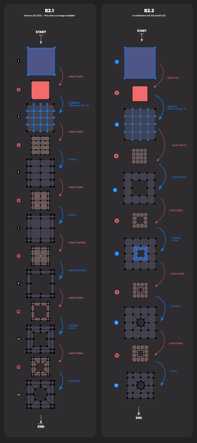
image 21
If we focus only on the inner part of the the topologies, in steps 8-11 of B2.1 and in steps 4-7 of B2.2, we can see that these procedures here proceed analogously to the procedure B1.3, only there were no outer edges there. This is a case of topological (and procedural) “embedding”, as discussed in more detail in the chapter “Discussion” below.
PROCEDURE B3
And finally, here's the following task: we need to find a procedure B3 that’ll take us from the starting topology (left) to the target topology (right):
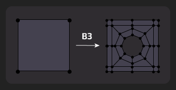
image 22
The resulting topology is similar to B2 (see the procedure by Arrimus 3D above), but this one, demonstrated by Josh Gambrell (Gambrell, 2020), has additional edges around the hole.
Just as in the case of the Lepiller’s procedure (A.1), this procedure is intended by the author for curved surfaces, and it would be impractical to use it on simple planar configurations such as the ones I’m exploring here. However, just to demonstrate the potential variability of procedures, I’m presenting it here. Here it is (a long one):
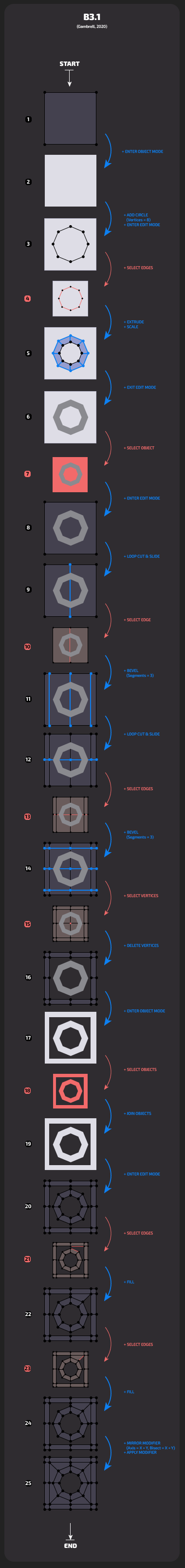
image 23
As noted above, in the planar case this is an impractical procedure, involving lots of steps and complex work on two separate models that get joined eventually.
DISCUSSION
We'll now turn to a discussion of several issues that appeared repeatedly in the above presentations.
First, I've mentioned in presenting the procedures B1.2 and B1.3 that the following two operations may, when presented in the m-diagrams, seem equivalent, for there's in each case a single selection step (IMAGE 24):
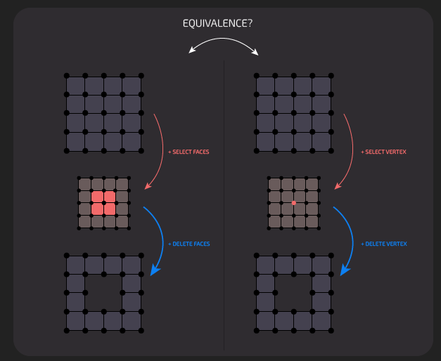
image 24
However, the above M-diagrams are imprecise. For simplicity's sake, they hide the actual sequence of four clicks in the case of selecting the faces.
That is, the selection of those faces should actually be expanded to four consecutive selection steps as this (IMAGE 25):
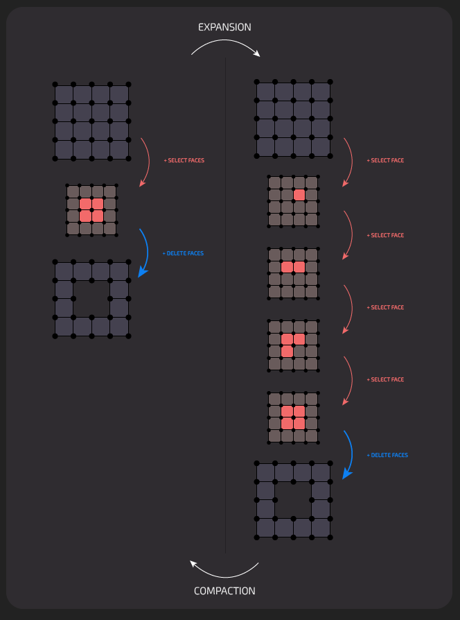
image 25
Thus, a procedure of selecting a single vertex can be considered an optimization of the procedure of selecting four faces:
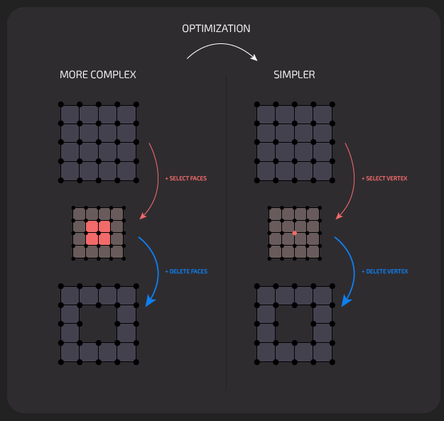
image 26
Another example of whether one procedure is less or more complex than another can be seen in the case of the procedures A.1 and A.2 above (IMAGE 17).
The latter (A.2) has more steps then the former (A.1), but we've discussed how using a modifier to make the simplest of subdivisions is an overkill, and therefore A.2 is not more complex than A.1:
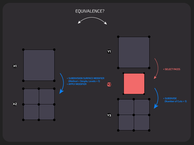
image 27
There is also a further issue with our M-diagrams: in Blender (the 3D software we've used as a base for the M-diagrams) once the operation has been applied on a selection of a topology's elements, the resulting topology has some of its elements already selected.
For example (IMAGE 28), Subdivide operation not only produces new topology, but it also selects the newly created elements for further operations:
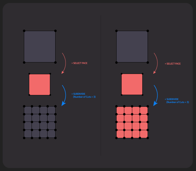
image 28
Another issue we encountered above (for example in the procedures B1.3, B2.1, and B2.2) is the "embedding" of a certain topological procedure into a local subtopology of a larger topology. In IMAGE 29, we can see how the X-procedure is embedded locally in the Y-procedure.
The reverse of this embedding is the "extraction" or "isolation" of a local subtopological procedure to a self-contained topoloogical procedure.

image 29
The last thing to mention, is that the above procedures, and especially the variants of the same procedure, can perhaps be grouped in a single branching m-diagram, such as the ones in IMAGES 30 and 31.
The first one (IMAGE 30) presents two sub-procedures (or: two threads) with a common pre-procedure (or: head) and a common post-procedure (or: tail). This is the case when we're grouping the various versions of a certain procedure into a single m-diagram.
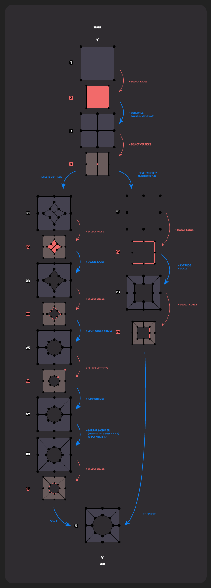
image 30
The other situation is the grouping of different procedures (that is, procedures with different result topologies) in a single m-diagram. In such case we often have a same pre-procedure (head), even though in the folowing the sub-procedures (threads) diverge (IMAGE 31).
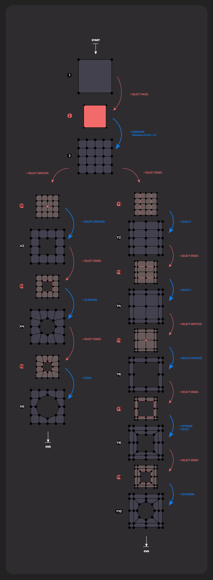
image 31
CONCLUSIONS
So, to conclude in a sort of a general overview, we can say here that the above topological procedures have the following three properties:
(1) These procedures are strictly linear. Even though above (IMAGES 30 and 31) we’ve drawn m-diagrams where there were two threads (two sub-procedures) branching out of a common (pre)procedure, when modelling, a 3D modeler is only proceeding along one such thread at a time, and eventually returns back to the branching point by a series of undos to, then, proceed along the other thread.
(2) These procedures proceed in a very regular alternation of “result steps” vs. “selection/operation steps”. That is, in order to alter a given topology, certain elements of it have to be selected and then modified, which we represent in the m-diagrams as a separate intermediate state, and these intermediate states are necessary to make clear what is actually the input of an operation and what operation is done to them.
There are exceptions to this: we’ve noted in the “Discussion” that, at least in Blender, topological operations not only produce new topologies from selected elements of the previous topology, but these operations also select the newly created topology's elements for further operations. This way it is not always necessary to have intermediate selection steps. Also, applying modifiers can have implicit selections, done under-the-hood by the modifier, without requiring a 3D modeler to make that selection choice by himself/herself.
(3) Finally, the measure of the complexity of a particular procedure is very much subjective, since we’re interested here in what is more complex for a human 3D modeler, not for the computer. That is, these procedures are intuitive (artistic) procedures, and we would like to provide a phenomenological, rather than purely technical definition of their complexity. This doesn’t mean that such complexity can’t be measured more precisely (mathematically), but that’s not our task here.
In evaluating a complexity of a procedure, we need to take into account (3.1) the number of steps it takes to complete a procedure (the obvious part), (3.2) the complexity of the applied selection/operation step (that is, the number of clicks to select the necessary elements, or the number of parameters in the modifier, etc.), and (3.3) the familiarity, habits, and preferences of a 3D modeller doing the modelling.
3D modelers that are used to certain modeling routines may find a particular topological procedure simpler (easier) if it can be accomplished the way they (these 3D modelers) are used to make their 3D models, even if these routines are formally more complex. For example, a procedure that is completed in more steps than another one may still be evaluated by a 3D modeler as the better or easier one, given that he/she has a routine or a habit or a preference of using it.
Another example is that the complexity of a procedure is very much goal-relative, that is, for curved surfaces a more complex algorithm may be the better (or the only) solution.
For this phenomenological evaluation of the complexity, the implementation details (that is the way a particular operation is implemented in a particular 3D software) can, on the one side, be disregarded, for only the simplicity of using the operation is important for a 3D modeler, but, on the other hand, some operations may be slower to actually perform on the computer (for example when working with a highly subdivided high-poly mesh), so the implementation can become phenomenologically critical.
Also, operations may be different and variously handy in different 3D applications, but on a certain general (more abstract) level, this can be ignored.
As mentioned in the "Introduction", none of the above conclusions suggests a normative “right”, “correct”, or absolutely “better” way of 3D modeling. On the contrary, instead of prescribing, they present a variety of routines done differently by different 3D modelers for different 3D modeling purposes.
The 3D modeling task can almost always be solved in several different ways, and the decision about which of these ways is the best way is best left to the 3D modeler in the particular situation.
However, as also mentioned in the “Introduction”, every 3D modeler can profit from knowing the comparative details of the procedures he/she uses.
CHALLENGES
I present here two challenges for 3D modelers who have read the above text. One of the challenges is easier (Challenge 1) and the other is harder (Challenge 2).
Here they are:
CHALLENGE 1 Can you find a simpler topological procedure for the same task as that of the procedure B3.1 above? (The easier challenge.)
CHALLENGE 2 Can you find a simpler topological procedure for the same task as that of the procedure A.2 above? (The harder challenge.)
REFERENCES
(Arrimus 3D, 2021) = Arrimus 3D, “Classic Topo Problem #10: Isolating Problem Areas”, published: 2021-09-22, retrieved: 2021-10-10
(Blender Secrets, 2020) = Blender Secrets, “Daily Blender Secrets: 10 Ways to Cut a Hole in Blender”, published: 2020-04-03, retrieved: 2021-10-10
(Blender Time, 2019A) = Blender Time, “Cut Hole on a Cube. SubD. Hard Surface Modeling - Blender 2.80”, published: 2019-01-29, retrieved: 2021-10-13
(Blender Time, 2019B) = Blender Time, “Blender 2.80 - Hole on Curved Surface. SubD Modeling”, published: 2019-01-31, retrieved 2021-10-14
(Evermotion, 2013) = Evermotion, “8 Techniques of Cutting Holes in Blender”, published: 2013-08-06, retrieved: 2021-10-14
(Flipped Normals, 2018) = Flipped Normals, “Hard Surface Modeling Essentials: Curved Surfaces”, published: 2018-08-23, retrieved: 2021-10-16
(Gambrell, 2020) = Gambrell, Josh, “The Right Way to Cut Holes in Surfaces in Blender”, published: 2020-04-20, retrieved: 2021-10-10
(Geis, 2020) = Geis, Justin (The CG Essentials), “3 Ways to Cut Holes in Objects in Blender”, published: 2020-03-09, retrieved: 2021-10-10
(Lepiller, 2020) = Lepiller, Cédric, “Speedflow Basics 15: Make Holes on Curved Surfaces”, published: 2020-03-06, retrieved: 2021-10-10
(Martin, 2015) = Martin, Johnson (Topology Guides), “Adding Holes to a Flat Surface”, published 2015-07-14, retrieved: 2022-04-08